Wargaming Insights: Cost of Ineffective Incident Response

How incomplete remediation can tilt the odds in the attacker’s favor

Introduction

In the first article of our Wargaming Insights series, we used a Markov Chain to model a simple attack scenario. We then compared two strategies Defense-in-Depth (preventive) and Detection & Response (reactive) and discussed their effectiveness.

Since our primary goal in that initial piece was to demonstrate the use of Markov processes, we intentionally over simplified the detection and incident response components of the model.

If you’d like to dive into the details of that simulation, you can check out the article below. It’s highly recommended for anyone looking to gain a solid understanding of the simulation approach we will use in this post.

One of the core assumptions in our initial simulation was this: once an incident response process is triggered after detecting an attack, it would always result in completely eradicating the attacker from the system. However, real-world incident response is far more complex than that.

Due to various factors that affect incident response such as limited visibility, access restrictions, poor planning, or miscommunication, remediation from an incident is not always 100% successful. For example, while a backdoor left by the attacker might be removed, the vulnerability that enabled the intrusion may remain unpatched or the passwords for compromised accounts may never be reset. In another scenario, during a spear-phishing campaign that infects multiple employees in the same organization the response team might fail to identify all victims and end up remediating only a single device.

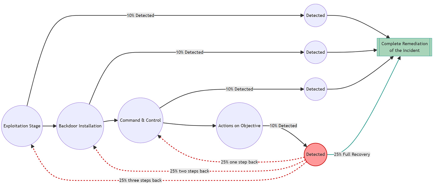
In such cases, even if the threat is detected and an incident response process is initiated, the attacker may not be fully removed from the environment. And more often than not, this leaves systems vulnerable to being compromised again. Therefore there is always a chance of an incomplete response during a real incident. If this happens the attacker moves back to one of the previous steps.

If we model this dynamic with a Markov chain we need to draw arrows from each detection step back to the earlier steps. So the probabilities after the “detected” step follow the red path shown in the graphic below.

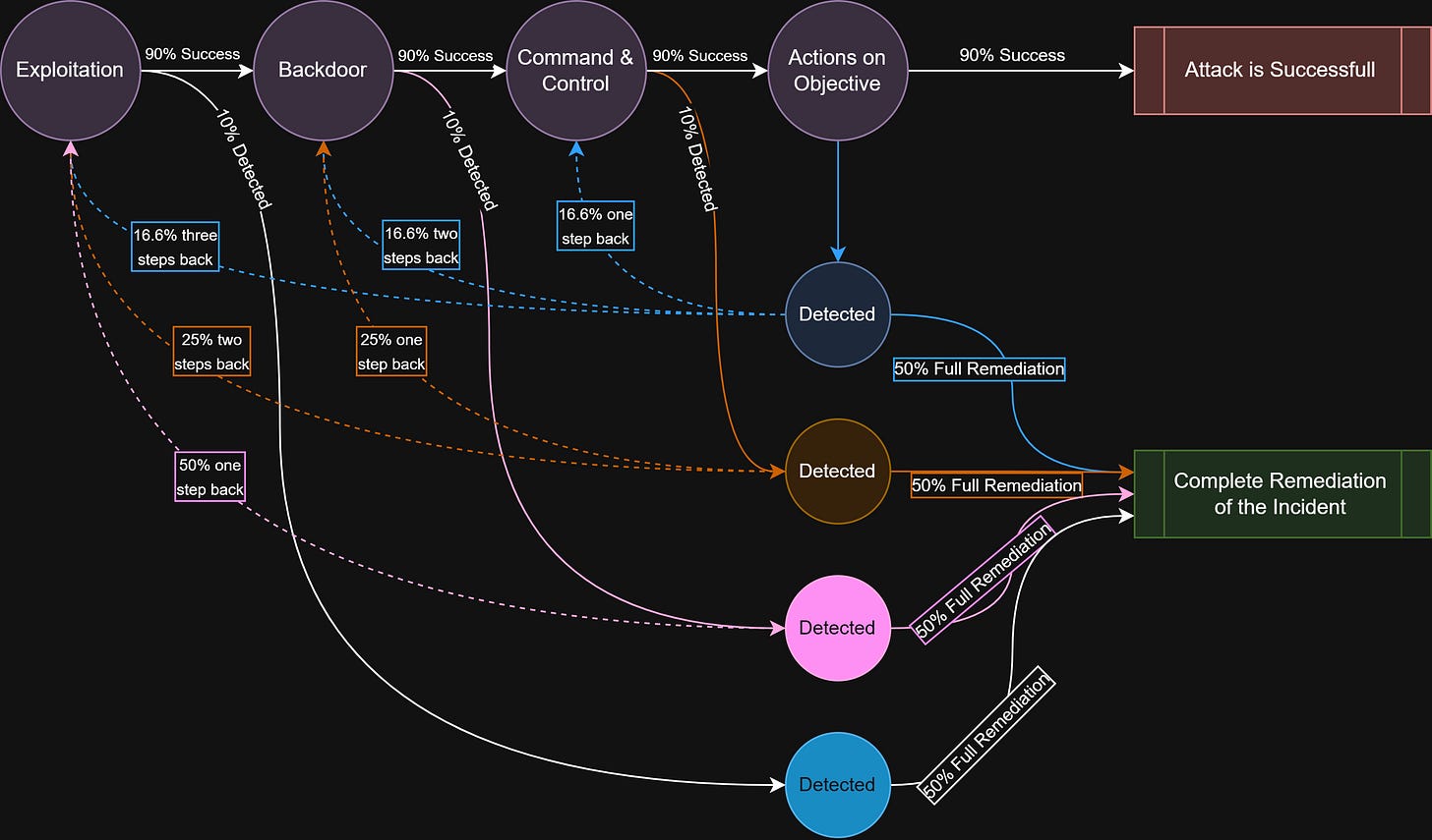
The full attack chain would look like the diagram below. After each detected step, there is an X% chance of complete remediation; otherwise the process randomly returns to one of the previous steps.

Disclaimer: Please note that the models in this post are deliberately oversimplified. They are designed to demonstrate the application of Markov Chains in simulation modeling. As such, they abstract away many real-world factors such as adaptive attacker behavior, response times, and cost of implementation. A more detailed model could be built to incorporate those factors, but that would go beyond the purpose of this post.

Modeling the Intrusion Chain

Now we will simulate our intrusion chain model using Python code. As you can see, since our new model includes backtrack connections, we can no longer perform a formal solution the way we did in the first article. Instead, we’ll run this model thousands of time in Python and observe the distribution of results. This method is also known as a Monte Carlo simulation.

As a first step, let’s define our intrusion chain. As an example, I selected the TTPs from one of the Lazarus Contagious Interview campaigns. The final stage of our attack is the ”Exfiltration over C2 Channel” step. In our simulation, an attacker who reaches this step will be considered successful.

# -----------------------------
# ATTACK CHAIN OF CONTAGIOUS INTERVIEW (Lazarus Group)
# -----------------------------
STATES = [
    “Initial Access – Phishing Attachment (T1566.001)”,
    “Execution – Mshta (T1170)”,
    “Persistence – Setup Folder (T1060)”,
    “Discovery - Process Discovery (T1057)”,
    “Collection – Data from Local System (T1005)”,
    “Exfiltration – Over C2 Channel (T1041)” # final state
]

When building the chain, an important point is to choose attack steps that can genuinely be treated as distinct from one another. Our simulation relies on the assumption that if an attacker is stopped at step N, they can fall back to step N–1. But if steps N and N–1 aren’t truly separate (if they operate together as part of the same activity) then the simulation becomes inaccurate.

For example, an attacker might use multiple techniques at once for C2 communication, such as Encrypted Channels and Non-Standard Port. Even though these are listed as separate MITRE ATT&CK techniques, in practice they are not independent steps. An attacker detected and pushed back at the “Non-Standard Port” stage wouldn’t realistically revert to an “Encrypted Channels” stage.

So these steps should be merged into a single consolidated phase (e.g: “Command and Control”) before constructing the chain.

---

Running the Monte Carlo Simulation

Below function will execute a single run of the Monte Carlo simulation. Conceptually, it works as follows:

• The attacker starts at the first step of the intrusion chain (state_index = 0).

• At each iteration, the model draws a random number to determine whether the attacker is detected or remains undetected.

• If the attacker is not detected, they simply advance to the next step in the chain.

• If the attacker is detected:

  • A second random draw decides whether the response leads to full remediation.

    • If yes, the simulation ends with a “Fully Remediated” result.

  • If remediation fails, the attacker is pushed back to a randomly selected earlier step.

    • The only exception is step 0: if detection happens there, we count it as full remediation.

• The simulation repeats this process until one of the following occurs:

  • The attacker reaches the final step → “Attack Successful”

  • A full remediation event is triggered → “Fully Remediated”

  • The loop hits the maximum step limit → “Timeout”

This structure lets the simulation capture the dynamics of a real intrusion where detection may push the attacker back rather than eliminate them outright.

# -----------------------------
# SIMULATION FUNCTION
# -----------------------------
def run_single_simulation(P_REMEDIATED, P_DETECTED, max_steps=2000):
    P_UNDETECTED = 1 - P_DETECTED
    state_index = 0
    steps = 0

    while steps < max_steps:
        steps += 1
        if state_index >= len(STATES) - 1:
            return “Attack Successful”

        rnd = np.random.rand()

        # 1) Undetected → move forward
        if rnd < P_UNDETECTED:
            state_index += 1
            continue
        else:
            # detected → full remediation or partial remediation
            rnd2 = np.random.rand()
            if rnd2 < P_REMEDIATED:
                return “Fully Remediated”
            else:
                if state_index == 0:
                    return “Fully Remediated”
                state_index = np.random.choice(np.arange(0, state_index))

    return “Timeout”

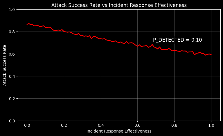
Let’s run our simulation using a baseline assumption of a 10% detection probability per step. In each simulation batch, we increase the incident response effectiveness by 1%, and we repeat this process until it reaches 100%. In other words, we’re trying to answer If I can detect 10% of all attack steps, how does improving incident response effectiveness affect the attacker’s overall success rate?

After running the simulation, we plot the results as shown below. As you can see, increasing incident response effectiveness reduces the attacker’s success rate from around 87% down to roughly 60%.

---

Simulating Various Detection Probabilities

How does the effectiveness of incident response influence attacker success across different detection probabilities? To explore this, we’ll run a series of simulations using the same model. This time, we’ll repeat the previous simulation multiple times, starting with a detection probability of 5% and increasing it by 5% in each iteration, continuing until we reach 50%.

A detection probability of 50% means that we can detect roughly one out of every two steps the attacker takes. In other words, if the entire intrusion chain consists of six steps, we would be able to detect about three of them. You can think of the detection probability as how many TTPs in the intrusion chain your detection rules are able to cover.

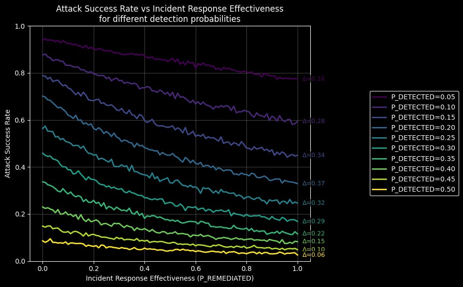
When we run the simulation repeatedly across this range of probabilities, we get the following results.

In each simulation, we represent the overall impact of incident response on attack success using the delta variable. For example in our first simulation (the dark purple line at the top), when the detection probability is 5%, increasing incident response effectiveness reduces the attacker’s chances of success by up to 16%. (Δ = 0.16)

When we test across different levels of detection coverage, we see that incident response effectiveness reduces the attacker’s success rate by an average of 22%. But more realistically, by somewhere between 25% and 35%.

A particularly interesting takeaway is that incident response effectiveness has relatively little impact on attack success at very low or very high detection rates (Δ = 0.16 and Δ = 0.06, respectively). In other words, incident response effectiveness becomes most critical when detection coverage is partial. This was a result I didn’t expect to see at the start of the analysis.

---

Conclusion

Our simulations yield the following key lessons for security leaders:

Prioritize improving detection coverage when it is very low.
If detection gaps are significant, enhancing coverage should be the first step, as improvements here provide the greatest reduction in attacker success.

Focus on incident response effectiveness when partial detection exists.
When planning against an intrusion chain with known detection gaps, prioritize improving the response playbook as it can significantly reduce the attacker’s chances of success. This may include automating key response actions to ensure timely and reliable mitigation.

Use simulations to guide strategy.
Monte Carlo-style simulations, as demonstrated here, provide a practical way to model the impact of different detection and response strategies. You may use these techniques to enable informed, data-driven decisions in complex security environments.

---

Limitations

The simulation presented in this article does not fully capture the dynamics of real-world incident response processes. In this sense, there are several important limitations to keep in mind:

1. Time-to-Respond is not modeled.
Our simulation assumes that as soon as a step of an attack is detected, the response can be executed immediately. In reality, detection, triage, investigation, and response can take days or even weeks to complete. This delay gives the attacker a critical window of opportunity to advance to subsequent steps. Therefore, when planning real-world incident response, the Time-to-Respond must be accounted for unless the response steps are fully automated.

2. Attacker adaptation is ignored.
The simulation assumes that if an attacker fails at a particular step, they will simply repeat the same actions as it did before. This overlooks the attacker’s ability to adapt. In reality, unless the attack itself is fully automated, attackers typically adjust their tactics when encountering failure and attempt alternative approaches. As a result, the detection probability assumed at the beginning of an intrusion gradually decreases as the attacker adapts. Addressing this limitation would require a more sophisticated modeling approach.

Ultimately, while simulations are very useful tools for decision-making, we must be aware of their limitations and continue refining our models to better capture real-world dynamics. Only then can we make truly informed and reliable security decisions.